
Transformer Categories
Transformer categories are a good starting point from which to explore the transformer list. Transformers are grouped in categories to help find a transformer relevant to the problem at hand.
Although all of them are important, the most commonly used transformers are found in these categories:
- Attributes: Operations for attribute/list management
- Calculated Values: Operations that return a calculated value
- Filters and Joins: Operations for dividing and merging data flows
- Geometries: Operations that create geometry or transform it to a different geometry type
- Spatial Analysis: Operations that return the result of a spatial analysis
- Strings: Operations that manipulate string contents, including dates
Several transformers can join data by matching attribute values (keys). Some of these are more oriented towards geometry, while others have a more SQL-like style. Some join streams of data within one workspace, while others join one stream of data to an external database.
a)FeatureMerger
The FeatureMerger is a transformer for joining two (or more) streams of data within a workspace based on a key field match.
Here, for example, a dataset of roads has a StreetId number. The FeatureMerger is being used to combine information from a spreadsheet of snowfall information onto the roads data:

The parameters dialog for the FeatureMerger looks like this:

This screenshot shows the join is made using StreetId as a key. All Requestor (Road) features that have a matching snowfall record are output through the Merged output port. All Road features without a match are output through the UnmergedRequestor port for inspection to determine why a match did not occur.
There are additional parameters to handle conflicts of information, duplicate keys, and whether to merge attributes only or geometry as well.
The FeatureMerger receives two streams of features via its input ports.
Requestor: Requestors are the features that will receive new attributes and/or geometry.
Supplier: Suppliers provide attributes and/or geometry to be merged onto the Requestors.
Matches between Requestor and Supplier are identified according to the Join On configuration in the parameters dialog. The Join conditions can be simple or complex, using attribute values, constants, functions, or a combination of any of these in expression form. Multiple join conditions can be defined (features must meet all conditions to match).

Examples
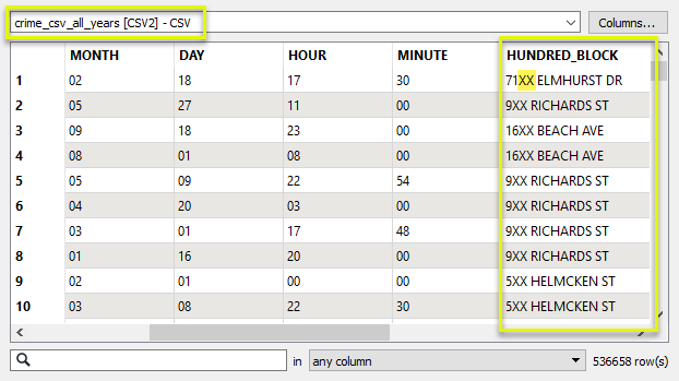
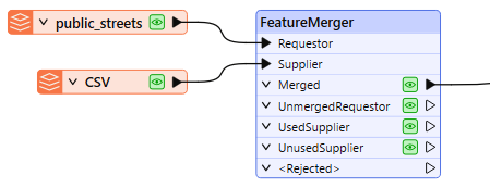
In this example, we have two datasets - a CSV text file of historical crime reports, and a shapefile of public streets. Both of the datasets have one piece of information in common, that is an address in the form of “hundred” block.
The FeatureJoiner would likely be more effective to do a simple attribute value join, however, the format of the address is slightly different in each dataset. The CSV data uses the string “XX” in place of zeroes in the address:
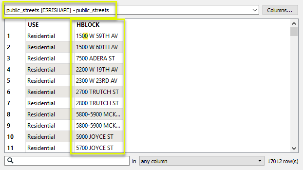
And the street data has the more conventional form, with zeroes:
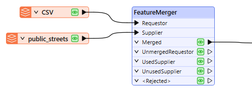
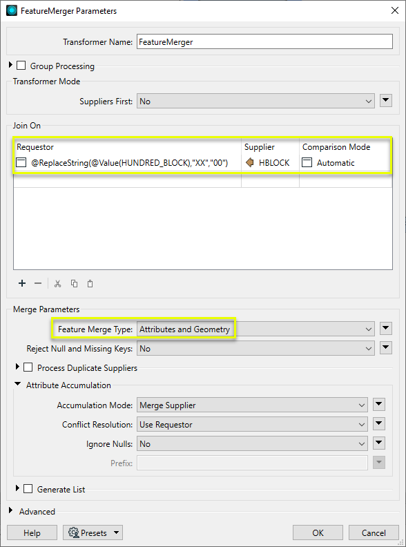
Our goal is to merge the street geometry onto the crime data - producing one output feature for each crime record. And so, The CSV data is routed into the Requestor input port, and the streets are routed into the Supplier port.
In the parameters dialog, we need to create a Join On pair of Requestor and Supplier values. As the format of the addresses is not identical, we will adjust one, constructing a key. With the assistance of the Text Editor, we create an expression that will replace the “XX” of the address with “00”, and so match the format of the street (Supplier) data.
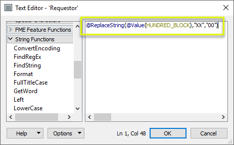
The other half of the pairing is the attribute value HBLOCK from the street data.
Feature Merge Type is set to Attributes and Geometry. The default values for Attribute Accumulation (Merge Supplier) will provide the correct results.
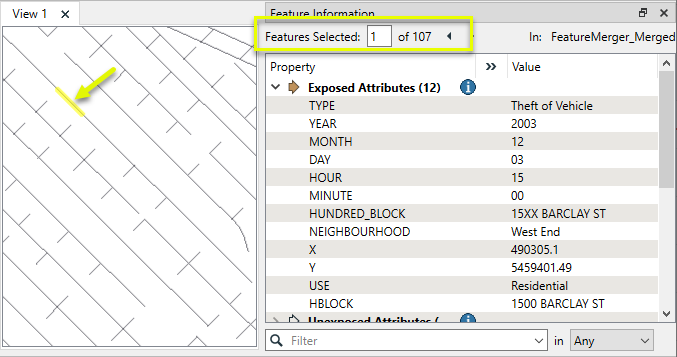
The Merged output contains crime records, now with geometry for the street and associated street attributes. Note that the address format was not actually changed by the constructed expression - it was just used for matching evaluation. In this location, 137 crime records were found. Each one now has (identical) geometry.
To see this example reversed - attaching all crime records to a single street - see the next example.
2) Example: Many-to-one merging to create a list attribute
In this example, we reverse the scenario in the above example. We want to merge all the historical crime records onto the street data, producing one record per street line segment (block), with a list attribute containing the crime data.
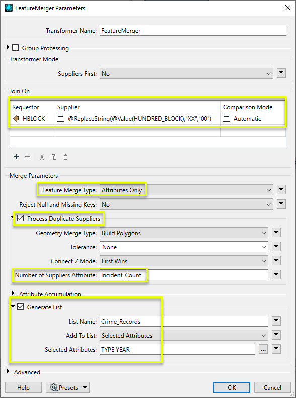
In this case, the streets are the Requestor features, and the crime data is the Supplier.
In the parameters dialog, we again create a Join On pair, using an expression to match the two (slightly different) hundred block formats. The Feature Merge Type is Attributes Only, as the Requestors (streets) already have the desired geometry.
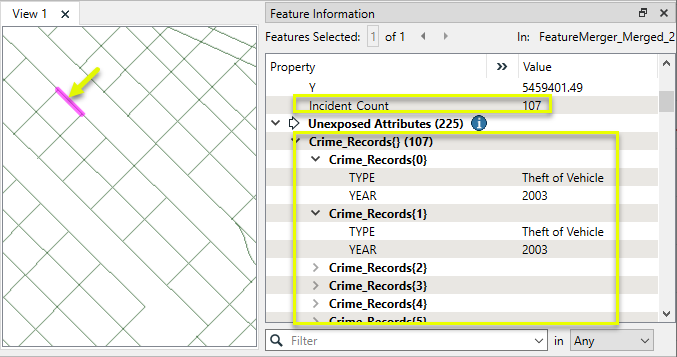
Process Duplicate Suppliers is enabled. Without this, the first match would be processed and the remainder discarded. A count of how many Suppliers (crimes) matched will be kept in the Number of Suppliers Attribute, named Incident_Count.
Generate List is enabled, and given the List Name of Crime_Records. We will add only Selected Attributes to the List, and choose TYPE and YEAR.
The Merged output features now have a list attribute, containing all matching records from the CSV. Note the Incident_Count attribute.
b) FeatureJoiner
The FeatureJoiner is another transformer for joining two streams of data within a workspace based on a key field match.

Here, for example, is the same Roads/Snowfall match in the FeatureJoiner. The parameters for the transformer looks like this:

As you can see, this transformer is based more on traditional SQL queries. The Join Mode parameter can take one of three values:
Join Mode | Joined Output |
|
|---|---|---|
| Inner |
|  |
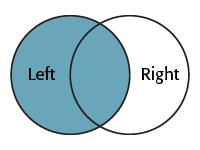
| Left |
|  |
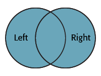
| Full |
|  |
Examples:-
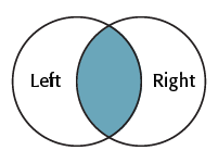
Inner Join


A Joined feature is produced each time a Left feature is matched to a Right feature through its keys. The number of output features produced will depend on whether or not multiple Left and Right features match.
The type of join is determined by the nature of the data used (it is not a parameter). Any of these types of joins may be produced by any of the Join Modes (Inner, Left, or Full).
Cardinality | Description | Output (assuming 1 key value) |
1:1 | One to One: If each Left feature has a single match among the Right features (for example a single point feature is mapped to an address table via a unique address ID key), this is a 1:1 match and produces a single Joined feature. | 1 Left matches 1 Right: 1 Joined Feature output |
1:M | One to Many: If each Left feature has multiple matches among the Right features (for example a single address record is mapped to a list of planning applications for that address), this is a 1:M (one-to-many) match and produces a Joined feature for every match that occurs. | 1 Left matches 10Right: 10 Joined Features output |
M:1 | Many to One: If multiple Left features match a single Right feature record (for example a number of addresses match to the same census data via a postal code field) this is a M:1 (many-to-one) match and produces a Joined feature for every match that occurs | 10 Left match 1 Right: 10 Joined Features output |
M:N | Many to Many: If multiple Left features match multiple Right features (for example a number of addresses match to a number of records for electrical power outages) this is a M:N (many-to-many) match and produces a Joined feature for every match that occurs. | 10 Left match 10 Right: 100 Joined Features output* *When all features have identical key values - all Left match all Right. |
- For simple joins, the FeatureJoiner may provide better performance than the FeatureMerger. However, the FeatureJoiner only accepts attribute values as keys and not constructed expressions, and does not support list attributes. Additionally, the FeatureMerger is able to (optionally) restrict output to one feature in the case of multiple matching Suppliers, whereas the FeatureJoiner will create multiple features for all matches.
- If the join requirements are simple, FeatureJoiner should give better performance.
- If join requirements are more complex, such as constructing keys, using expressions, naming conflict resolution, consider using the FeatureMerger.
- If you wish to get only one joined feature, regardless of the number of joins (1:M join produces 1 feature with a list of joins, rather than 1 feature for each join as the FeatureJoiner does), use the FeatureMerger.
- The FeatureJoiner does not perform some of the advanced list building or geometry handling operations that the FeatureMerger does, but these may be possible by using the FeatureJoiner plus other transformers.
- The FeatureMerger may be able to join features with different coordinate systems.
The DatabaseJoiner transformer is different to the FeatureMerger and FeatureJoiner because, instead of merging two streams of features, it merges one (or more) stream(s) of data with records from an external database.
Typical Uses
- Joining attributes from an external database table to features already in a workspace.

Here is the same example as for the FeatureMerger above. In this case, the roads features are obtaining snowfall data directly from a table in an Excel spreadsheet:

The parameters dialog for the DatabaseJoiner looks like this:

Again, StreetID is being used from both feature and database table to facilitate a merge between the two.
As with the other transformers, there are parameters to control the attributes that are accumulated and how conflicts are resolved.
Usage Notes
The DatabaseJoiner has a number of advantages over the FeatureMerger.
Firstly it has parameters to control how multiple matches are handled, as well as parameters for optimizing the database query.
Secondly, it allows features to be joined without having to read the entire dataset into a workspace. FME can just query the database and select the individual records it needs. This can improve performance greatly.
d) InlineQuerier
The InlineQuerier transformer accepts features from the workspace and generates a temporary database. With that database it's possible to apply any SQL commands required - including Joins - across a number of tables:
Typical Uses
- Performing SQL queries on any features, whether or not they originate from a SQL supporting format.
- Executing complex queries and joins without multiple transformers

The InlineQuerier has the distinct advantage of allowing its input to be reused multiple times in a single transformer; whereas multiple joins would otherwise require multiple FeatureJoiner transformers. However, there is a performance overhead involved in generating that initial database.
Example of Inner Joiner query:-
SELECT "Unique".* , "Sorted1".* FROM "Unique" INNER JOIN "Sorted1" ON "Unique"."name_data" = "Sorted1"."unparsed_name"
See the SQLite documentation for a detailed reference on the SQL Select statement syntax that is supported.
Usage Notes
- For complex joins using SQL syntax, or more than two input feature streams, consider using the InlineQuerier.
- Where multiple FeatureMergers are required, consider using the InlineQuerier instead.
- If all the data to be queried already exists in a SQL-capable data source, it is always more efficient to use the SQLCreator or SQLExecutor, which allows the queries and filtering of the data to be executed directly by the database before it enters the FME environment.
- To perform a join between features already in the workspace and data residing in an external database, consider the DatabaseJoiner.
- To perform a join where the Requestor key is a list attribute, consider using the ListBasedFeatureMerger.
- To join features on matching geometry, consider the Matcher. The FeatureMerger does not accept geometry as a key.

Transformer | Match By | Uses SQL Statements | Can Create List | Input Type | Notable | Description |
FeatureJoiner | Attributes | No | No | Features |
| Joins features by combining the attributes and/or geometry of features based on common key attribute values. Performs the equivalent of Inner, Left, and Full SQL joins. |
Attributes | No | Yes | Features |
| Merges the attributes and/or geometry of one set of features onto another set of features, based on matching key attribute values and expressions. | |
List Attribute to Single Attribute | No | Yes | Features |
| Merges the attributes and/or geometry of one set of features onto another set of features, based on matching list attribute values with key attribute values and expressions. | |
SQL query | Yes | No | Features |
| Creates a set of SQLite database tables from incoming features, executes SQL queries against them, and outputs the results as features. | |
SQL query | Yes | No | External DB |
| Generates FME features from the results of a SQL query executed once against a database. One FME feature is created for each row of the results of the SQL query. | |
SQL query | Yes | No | External DB |
| Executes SQL queries against a database. One query is issued to the database for each initiating feature that enters the transformer. Both the initiating features and the results of the query may be output as features. | |
Attributes | No | Yes | External DB and Features |
| Joins attributes from an external table to features already in a workspace, based on a common key or keys. SQL knowledge not required. Non-blocking transformer. | |
Geometry and/or Attributes | No | Yes | Features |
| Detects features that are matches of each other. Features are declared to match when they have matching geometry, matching attribute values, or both. A list of attributes which must differ between the features may also be specified. If matching on attributes only (not geometry), using the FeatureMerger or another method will give better performance. |
Multiple transformers can join data by spatial relationship. Which you use depends on the spatial relationship to be tested and your exact join requirements. The following are some of the key transformers.
a) Overlayers
There are a number of different "overlayer" transformers, each handling a different form of overlay.
For example, the PointOnAreaOverlayer carries out a spatial join on points that fall inside area (polygon) features. This operation is sometimes called a "Point in Polygon" overlay.
As the help explains, "each point receives the attributes of the area(s) it is contained in, and each containing area receives the attributes of each point it contains."

Here the TransitStation features are being provided with a postal code (CFSAUID) depending on which PostcodeBoundary polygon they fall inside.
The "_overlaps" attribute is another useful outcome of this transformer. It tells us how many polygons each station fell inside; in this case, overlapping postal codes might be spotted by a station having more than one overlap.
Conversely, the Area output would have an "_overlaps" attribute that would tell us how many stations fell inside each postal code.
1) PointOnAreaOverlayer :-
Performs a Point in Polygon overlay. Points may receive containing area attributes, and areas may receive contained point attributes (spatial join).
Typical Uses
- Finding which areas that points fall inside
- Finding which and how many points are contained within areas.

2) PointOnLineOverlayer:-
Performs a point-on-line overlay. Each input line is split at its closest place to any point within the specified point tolerance, and attributes may be shared between related points and lines (spatial join).
Typical Uses
- Splitting lines where they overlay points
- Identifying lines that intersect with a point
- Identifying points that fall on a line

3) PointOnPointOverlayer:-
Performs an overlay of points on points. Each point may receive attributes from any point within a specified distance (tolerance), performing a spatial join. Geometry is not altered.
Typical Uses
- Aggregating data from multiple points in the same location
- Combining attributes from different co-located point datasets
- Relating text or labels to point data
How does it work?
The PointOnPointOverlayer compares all point features that enter through the Point input port against each other. Each point may receive attributes from all other points located within the specified tolerance distance (a spatial join). Points also receive a count of the number of matched points encountered. Geometry is unaltered. Aggregates/multipoint geometries can either be deaggregated before processing or rejected.
In this example, we start with a single point dataset of reported crimes, over many years. The points are routed into the Point input port of the PointOnPointOverlayer.
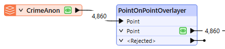
There are two tasks we want to accomplish.
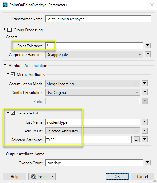
First, we want to count how many crimes were reported at any given location within the dataset. The Overlap Count Attribute will tell us how many other points were found within 2 meters of the location (as defined in the Point Tolerance parameter, with the data in a UTM projection, ground units in meters).
Second, we will build a list attribute that contains the type of each report in the location. We enable Generate List, and add the Selected Attribute “TYPE” to a list named IncidentType.
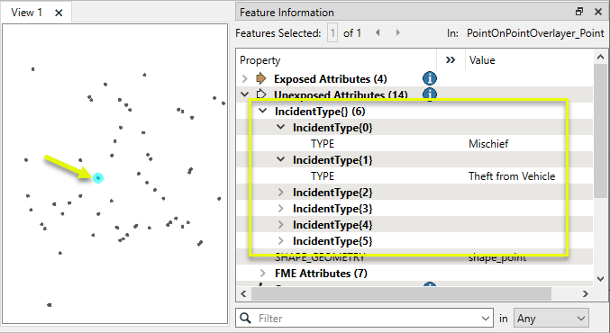
The points are output with no changes to their geometry, but with new attributes added. The example point selected now has an _overlaps value of 8, indicating that eight points (crime reports) in total are at this location.
The IncidentType list collects the Type attribute from each of the matching points.
b) NeighborFinder
The NeighborFinder transformer carries out a spatial join based on a proximity relationship.
Description
The NeighborFinder locates the nearest 'candidate' feature to a 'base' feature and copies the candidates attributes over to the base feature.
Typical Uses
- Identifying the nearest feature(s)
- Identifying features within a specified distance
- Adding a point closest to a candidate (such as adding a point on a railway track at the closest point to a station)
- Finding the closest feature in a certain direction (by filtering the resulting candidate angle)
- Calculating clusters or density by counting neighbors within a set distance
How Does It Works?
The NeighborFinder generally takes in two sets of features - Base and Candidate. For each Base feature, the transformer checks the Candidates for matches, based on proximity and parameter selections. It may check for the closest Candidate feature, or a fixed maximum number of closest Candidates, or all Candidates that fall within a specified distance of the Base feature.
Attributes from one matching Candidate are added to the Base features, including:
- Attributes from matching Candidate
- Calculated attributes containing distance, angle, and coordinates of matches
- Coordinates of the interpolated point on the Base that is closest to the Candidate
Attributes from multiple matching Candidates may be stored in a List attribute.
Output includes MatchedBase features with these new attributes, Unmatched Base features (unchanged), and Unmatched Candidates(unchanged).
The NeighborFinder works with 2D geometries only; if an input geometry is 3D, its z-coordinate will be ignored. The transformer has full support for points, lines, arcs, ellipses, polygons, and donuts, and has limited support for other types of geometry. Polygons, ellipses and donuts may be processed as lines or areas, depending on user selection.
Candidates Only Mode
The NeighborFinder can be used in a Candidates Only mode, in which only Candidate input features are considered. In this mode, each feature is considered the Base in turn, and compared to all other Candidates (but not itself). Attribute sharing and Output behavior are the same as above.
Candidates-Only Mode is enabled with the Input parameter. When Input is set to Candidates Only, the Base input port is removed.
All CANDIDATEs will be compared with all other CANDIDATEs, but will not be compared to themselves.

Here the NeighborFinder is being used to identify the closest fire hall to each transit station:

The fire hall number, name, address, and phone number attributes are merged onto each Facility feature along with a number of useful attributes (not all shown) recording the X/Y coordinate, direction, and distance of the closest fire hall.
The parameters of the NeighborFinder includes the ability to specify a maximum distance for the relationship, or the maximum number of neighbors to find.
NeighborFinder and Format Attributes
Problems may occur when the base and candidate features have different geometry types.
For example, when using point features as the base and line features as the candidate all candidate attributes are copied to the nearest base feature. This includes 'format attributes' such as fme_geometry. So after processing the base point features now have a geometry type of mif_polyline (for example) when they ought to be mif_point
Performance Tip
The greater the max distance, and the more features that fall within it, the longer the process will take. Basically we create a list of features to consider and compare them, vertex by vertex, candidate against base, to find the shortest distance between the two features. This is a computationally intense step.
To improve performance you may get better results by using more than one NeighbourFinder.
For example, you believe most candidates will be within 10m of the base features, but want to set a maximum of 1000m to be absolutely sure.
- Set a NeighborFinder with a 10m max distance
- Any UNMATCHED_BASE features go into a second NeighborFinder with a 1000m max distance
That way the majority of base features are only compared against a much smaller subset of candidates.
The effect is greatest when most candidates are very close, but some may be very far.
c) FeatureReader
The FeatureReader is the spatial equivalent of the DatabaseJoiner transformer. It reads from an external dataset and forms a match based on a spatial relationship between the initiating feature and features in that dataset.
The FeatureReader transformer is one that acts – as the name suggests – as a reader in itself. Each incoming feature triggers a query to a database (or, in fact, any dataset) that can include both spatial and non-spatial data. This way queries can be carried out mid-translation, rather than through Reader parameters.
Incoming features are known as Initiators. Each of initiator feature causes a single query to be carried out through the reader. The query can be an attribute query, spatial query or a combination of the two.

One difference is that the output is not the original feature, but the queried feature; hence the name FeatureReader.
Reads features from any FME-supported format. A complete read is done for each feature that enters the Initiator port. The features resulting from the read are output either through named output ports or through the generic output port.
The features read can be constrained by specifying a WHERE clause or a spatial filter for formats that support them. Most reader settings and constraints can be configured dynamically from attribute values on the input features.
Additionally, a schema feature representing the feature type definition is output for each encountered feature type. The schema features can be used to configure feature type definitions for dynamic writing.

For example, here the FeatureReader is being used to carry out the same overlay of transit stations and postal codes. The PostcodeBoundaries features are read into the workspace and used as a means to spatially query TransitStations (a table in a Geodatabase). The stations are retrieved with the attributes of the postcode feature they fall inside.
This also acts as a form of filter, as stations are not outputted unless they fall inside the postcode boundary.
d) SpatialFilter
The SpatialFilter - as its name suggests - filters data according to a spatial relationship. However, it does also merge attributes from one feature to another, therefore can be said to be a type of Spatial Join.
Spatial relationships (also known as predicates) define how two or more spatial features interact with each other.
For example, two features might intersect each other (or not, in which case they are disjoint), they might touch each other (where the boundaries intersect, but the interiors do not), or one feature might contain a second feature (which itself is therefore within the first feature).

The important part is to connect both Passed and Failed output ports unless you do want to also filter the data.
How does it work?
The SpatialFilter compares two sets of features to see if their spatial relationships meet selected test conditions. The features being tested (Candidate features) are identified as having Passed or Failed the test.
For example, if you have a roads dataset (lines), and wanted to extract all the roads that passed through parks (polygons), you would direct the roads into the Candidate input port, and the parks into the Filter input port.
By selecting the test conditions Filter OGC-Intersects Candidate and Filter OGC-Contains Candidate, any road lines that fall within the parks or intersect the parks would be output via the Passed output port, and the remainder would exit through the Failed output port. You could simultaneously extract an attribute from the park polygon – park name, for example – and add it to the line feature.
e) Clipper
Performs a geometric clipping operation (sometimes called a cookie cutter). Most geometry types can be clipped by an area, and some may also be clipped by a solid. Attributes may be shared between objects (spatial join).
Typical Uses
- Identifying where points, lines, or areas fall inside, outside, and intersect with one or more reference areas (Clippers), and modifying their geometry and attributes accordingly.
- Clipping features to perform calculations by Clipper area
- Clipping rasters or point clouds to a regular or irregular area of interest
- Clipping features to a map boundary for aesthetics.
The Clipper takes in two sets of features:
- Clippers, which will be overlaid on other features to identify which of those features fall inside or outside the Clippers, and split those features where they cross the boundaries of the Clippers.
The geometry of the Clippers is unchanged, and they are discarded after use and not output from the Clipper transformer. - Clippees, which are compared to the Clippers, and split into multiple sections along the Clipper boundaries if necessary. Each section is output as either falling Inside or Outside the Clipper. They may also receive attributes from the Clippers (spatial join).
Clippee geometry is only altered if it intersects with a Clipper. If it falls wholly inside or outside the Clipper, it is designated as such and output with its geometry untouched.
Output features receive a new Clipped Indicator Attribute (default name _clipped), which is set to “yes” for features that have been segmented, enabling differentiation between features that were wholly inside or outside the clip boundaries and those that intersected the Clipper feature(s) and so were modified.
The Clipper works on many geometry types. This diagram illustrates area-on-line and area-on-area vector clipping results.
- (1) is a single area Clipper (in blue).
- (2) are the Clippees, a red line that crosses the Clipper (1), and red area that partially overlays the Clipper (1).
Both the line and area Clippees are split where they cross the Clipper boundary, and the results are output:
- (3) Portions of Clippees that fall Inside the Clipper (red only)
- (4) Portions of Clippees that fall Outside the Clipper (red only)

f) Matcher
Detects features that are matches of each other. Features are declared to match when they have matching geometry, matching attribute values, or both. A list of attributes which must differ between the features may also be specified.
How does it work?
The Matcher can receive any number of input feature streams. All features are compared against all other features, and matches are identified based on the parameters defined.
Options for matching include geometry and/or attributes, and you may also define attributes that must differ.
All features that find a match are output via the Matched port (that is, if two features match each other, both of them are output here). Each set of matches is given a new numeric Match ID attribute that can be used to identify them as a matching group.
A single copy of each set of matched features is sent to the SingleMatched port. The attributes on these features are merged on to one output feature. Using this port, the Matcher is capable of doing multi-feature merging using geometry as the key. This complements the FeatureMerger, which only accepts attributes, and not geometries, as keys.
Usage Notes
- The ChangeDetector provides an alternative (but less general) approach which may be more convenient for certain applications.
- When looking for matches based only on attributes, consider the FeatureJoiner or FeatureMerger for better performance.
- Oriented points are supported, however, precision loss when converting between orientation representations will often cause the ChangeDetector and Matcher to identify two oriented points as Updated/NotMatched unless Lenient Geometry Matching is enabled.
Features that do not find a match are output via the NotMatched port.
f) Intersector:-
Computes intersections between all input features, breaking lines and polygons wherever an intersection occurs and creating nodes at those locations. Overlapping segments are reduced to one segment before being output.
Typical Uses
- Identifying intersections within a dataset
- Reducing geometry to line segments
- Intersecting linear features at junctions to create clean topology
- Cutting overshoots at their intersection
- Creating points (nodes) at intersections to find likely features
The Intersector takes all input features and compares them to each other. Features are split wherever there is an intersection. Split features receive attributes from intersecting features (a spatial join), and the number of overlaps encountered and segments created is counted.
Intersected segments are output, as well as nodes (point features) placed at the location of each intersection. Optionally, a list attribute can be created which will retain attributes for multiple matches.

Aggregates can either be deaggregated before processing or rejected.
Example: Finding intersections and building lists
In this example, we start with a dataset of street centerlines. The street geometry is as contiguous as possible - the line segments are not broken at intersections, as shown here with a selected street highlighted in yellow. We want to create intersections, and find out which streets cross at those intersections, using a list attribute.

The street dataset set is routed into an Intersector.

In the Intersector parameters dialog, Generate List is enabled. The list is named Intersections, and one selected attribute - NAME - will be captured in the new list.

At each intersection of the lines, they are split, and a node is placed at the intersection. The nodes have a list called Intersections, which contains the NAME attribute we requested, as well as the angle and direction of line it is referring to.
The selected node shown here has four items in the list, as four line segments converge at that point - Haro St incoming and outgoing, and Jervis St incoming and outgoing.

g) Topology Builder:-
Network topology is made from a network of nodes and lines that is maintained throughout an area. The vitality of topological networks relies on consistent and connective geometry. Topology is often applied to transportation datasets, to ensure certain logic is being followed
Computes topology on input point, line, and/or area features, and outputs significant nodes, edges, and faces with attributes describing topological relationships.
What is required before you can build a topological network?
In order to successfully generate a network topology, some conditions must be met.
Lines must touch (be snapped) at an end vertex - first or last.
Lines must be split at junctions. The TopologyBuilder can automate this process, but will not consider z-values (and so may not produce correct results for overpasses/underpasses, for example.)
A junction at an interior vertex (not an end vertex) produces a complex edge, which is not supported.
- The TopologyBuilder will not correct data - it will only find relationships and intersections that exist.
- Typical Uses
- Computing topological relationships on vector features
- Finding intersections
The TopologyBuilder computes topology on input point, line, and/or area features.
Topologically significant nodes and lines are computed using all input features and output with additional attributes which describe the topological relationships. The TopologyBuilder will intersect the inputs before building topology, provided the Generate From advanced parameter is set to End Nodes and Intersections. It takes any data and constructs the resulting topology after computing any intersections present in the input data.
It outputs the significant Nodes (points) and Edges (lines) with attributes describing their topological relationships. Faces (areas) are output with information about the Edges which form them.
This transformer is typically used to determine topological relationships to aid in decision making in later transformers.

* Red line indicates direction of flow.
Valency refers to the number of line segments attached to a node.

Example: Computing topology on street centerlines
In this example, we start with a set of whole street centerlines, which are not split into individual features at intersections.

The features are routed into a TopologyBuilder.

The default parameter settings will produce correct and useful results. It is worth noting that the default setting of Generate From is left as End Nodes and Intersections, and so will create intersections where lines cross.

At intersections, the lines are split and nodes are created. Nodes receive attributes about connecting edge (line) features, including identifier and angle.

The Edges (line segments) also receive attributes about their relationship with adjacent features.

Spatial Transformers Comparison Matrix

Transformer | Can Merge Attributes | Alters Geometry | Counts Related Features | Creates List | Supported Types* | Recommended For |
Yes | No | No | No |
|
| |
Yes | No | Yes | Yes |
|
| |
Yes | Yes | Yes | Yes |
|
| |
Yes | Yes | Yes | Yes |
|
| |
Yes | Yes | Yes | Yes |
|
| |
Yes | No | Yes | Yes |
|
| |
Yes | Yes | Yes | Yes |
|
| |
Yes | No | Yes | Yes |
|
| |
Yes | Yes | Yes | Yes |
|
| |
Clipper | Yes | Yes | No | No |
|
|
Yes | In some cases | No | Yes |
|
| |
Yes | Yes | No | Yes |
|
|


No comments:
Post a Comment